Training a VAE on Super Mario Bros and playing its levels

May 23, 2022

We recently open sourced an implementation of a categorical VAE trained on levels from the classic game Super Mario Bros. In this blogpost I expand on how it works, and how it can be used to play content directly from latent space. This blogpost covers how the model is defined and how the simulator we provide can be used to automatically extract things like how many jumps were performed, or whether the level is solvable by an artificial agent.

This post assumes you know a little bit about about how Variational Autoencoders work (e.g. what the ELBO loss is), that you know how to use Python up to an intermediate level, and that’s it!

The data: levels from Super Mario Bros #

In the Video Game Level Corpus you can find post-processed versions of content for several different games, including Super Mario Bros 1 and 2. These processed levels, in the case of SMB, are long text files with 14 rows and \(n\) columns. All sprites are encoded using a unique token: "-" represents empty space, "X" represents the floor, and so on. There are 11 unique sprites in total in the case of SMB 1.

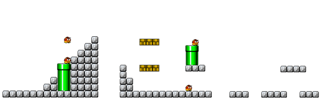
We split them into 14x14 chuncks by rolling a window across all levels. In total, we have 2713 levels saved in ./data/all_levels_onehot.npz as (n_sprites=11, height=14, width=14) arrays. To load them, you can run np.load(that_path)["levels"]. Here are three random examples of said levels, visualized using some of the tools provided in the repo:

The model: a categorical VAE #

We used a simple Variational Autoencoder with multi-layer perceptrons for both the encoder and the decoder. Remember that a Variational Autoencoder approximates two distributions \(q(z|x)\) and \(p(x|z)\) using these networks. The first distribution models the relationship between latent codes \(z\) and data \(x\) by proposing a variational posterior (usually a multivariate Normal), starting also with a Normal prior \(p(z)\) .

The other one, \(p(x|z)\) , models the distribution of our data given a particular latent code. In our case, this distribution is categorical, or discrete. We have \(11\) tokens (each one of the sprites), and we are modelling the probability of each one of them.

With PyTorch Distributions, implementing Variational Autoencoders is easy!¹ We model the encoder using the following layers:

self.encoder = nn.Sequential(
    nn.Linear(self.input_dim, 512),  # self.input_dim = 14 x 14 x 11
    nn.Tanh(),
    nn.Linear(512, 256),
    nn.Tanh(),
    nn.Linear(256, 128),
    nn.Tanh(),
).to(self.device)
self.enc_mu = nn.Sequential(nn.Linear(128, z_dim)).to(self.device)
self.enc_var = nn.Sequential(nn.Linear(128, z_dim)).to(self.device)

That way, when we encode we can return a Normal distribution:

def encode(self, x: torch.Tensor) -> Normal:
    # Returns q(z | x) = Normal(mu, sigma)
    x = x.view(-1, self.input_dim).to(self.device)
    result = self.encoder(x)
    mu = self.enc_mu(result)
    log_var = self.enc_var(result)

    q_z_given_x = Normal(mu, torch.exp(0.5 * log_var))

    return q_z_given_x

In other words, we encode first to a 128-sized layer, and we use this to output the mean and the log-variance of the Normal distribution that parametrizes the distribution \(q(z|x)\) of our latent variables given some data. This distribution is a Normal, which is a class inside torch.distributions.

Something similar can be done with the decoder:

# Going from the latent dim to one-hot space.
self.decoder = nn.Sequential(
    nn.Linear(self.z_dim, 256),
    nn.Tanh(),
    nn.Linear(256, 512),
    nn.Tanh(),
    nn.Linear(512, self.input_dim),
).to(self.device)

using the Categorical distribution inside torch:

def decode(self, z: t.Tensor) -> Categorical:
    # Returns p(x | z) = Cat(logits=what the decoder network says)
    logits = self.decoder(z)
    p_x_given_z = Categorical(
        logits=logits.reshape(-1, self.h, self.w, self.n_sprites)
    )

    return p_x_given_z

Notice how this allows us to write the ELBO loss using only probabilistic terms:

def elbo_loss_function(
    self, x: torch.Tensor, q_z_given_x: Distribution, p_x_given_z: Distribution
) -> torch.Tensor:
    # transform data from one-hot to integers
    x_ = x.to(self.device).argmax(dim=1)  

    # Computing the reconstruction loss (i.e. neg log likelihood)
    rec_loss = -p_x_given_z.log_prob(x_).sum(dim=(1, 2))

    # Computing the KL divergence (self.p_z is a unit Normal prior)
    kld = kl_divergence(q_z_given_x, self.p_z).sum(dim=1)  # b

    return (rec_loss + kld).mean()

The upside of using torch.distributions is that you could change the distribution of your data with minimal changes to this error function. The log_prob method works as a multiclass cross-entropy loss function when p_x_given_z is the categorical, but it could easily have been a MSE loss if we had used the Normal distribution to model our data instead.

You can find the entire description of the model here. In the repo, you can find an already-trained model under ./models/example.pt. If you wanna see the entire latent space, take a look at this image.

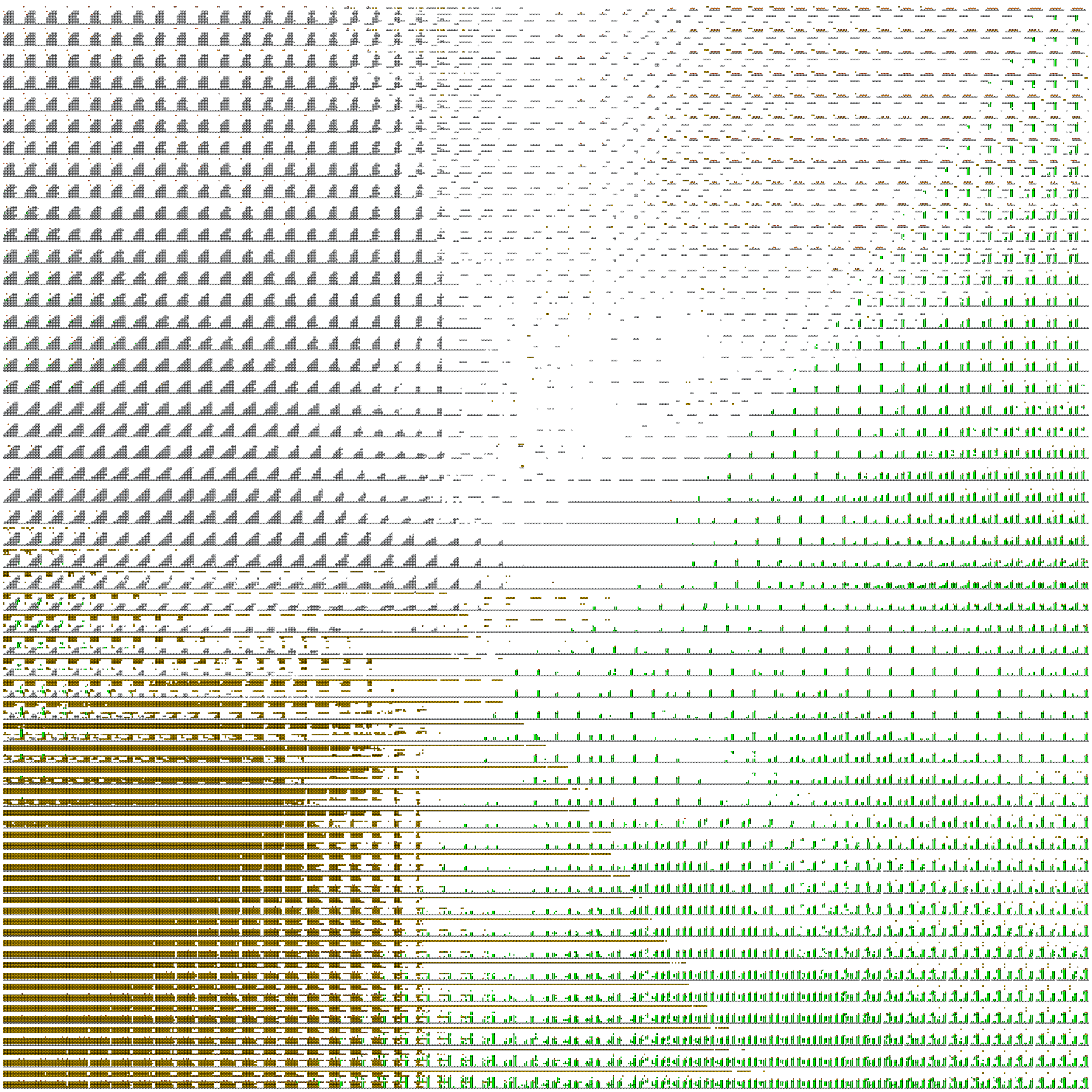
The simulator: the Mario AI competition #

In 2009, Robin Baumgarten’s won the Mario AI competition with a super-human agent based on the A star algorithm.² A modified version of the simulator used for the competition is available in the MarioGAN repository. This simulator gives you access to some statistics from the agent’s runs. We did a small modification to extract the data as JSONs and then compiled it. This compiled version can be found in the repository as simulator.jar. We used OpenJDK version 15.0.2 to run our experiments.

The class geometry.PlayLevel inside simulator.jar lets you play a given level (given as a command-line argument) using your keyboard, and geometry.EvalLevel uses Baumgarten’s A star agent to simulate the level and give you back telemetrics as JSON. These telemetrics count how much of the level was traversed, for how long, how many jumps were performed… The entire description can be found here.

In the repo, you can find the simulator and a Python interface (in simulator.py). This script implements utilities for sending levels decoded from the latent space to the compiled simulator. Here, I will provide a quick overview of how to use this interface, but I won’t dive into the details of how it was implemented. I know you’re a smart cookie, and you could go through the source code in simulator.py if you wanted to learn about how it works under the hood.

Let me give you an example using the network I provide under ./models/example.pt. We will implement a function that loads the network, decodes \(n_l\) random levels, concatenates them, and lets you play them. We can start by loading up the model:

from pathlib import Path

import torch

from vae import VAEMario

# The root path of the repo
ROOT_DIR = Path(__file__).parent.resolve()

# Creating an instance of the model with the default hyperparams
model = VAEMario()

# Loading the trained model
model.load_state_dict(torch.load(ROOT_DIR / "models" / "example.pt"))
model.eval()

Now we can get some random levels by sampling a normal distribution, decoding them to get \(p(x|z)\) , and choosing the most probable sprites:

# Defining how many levels
n_levels = 5

# The latent dim of the model (2, by default)
latent_dim = model.z_dim

# Getting {n_levels} random latent codes.
random_zs = torch.randn((n_levels, latent_dim))

# Decoding them to a categorical distribution
p_x_given_z = model.decode(random_zs)

# Levels (taking the argmax of the sprite probabilities)
levels = p_x_given_z.probs.argmax(dim=-1)

# Concatenating them horizontally
one_large_level = torch.hstack([lvl for lvl in levels])

At this point, one_large_level is a tensor of integers, each one of them representing the ID of a sprite³. Finally, simulate.py has a function that lets you run a level like this:

# A function in the simulator interface that lets
# you play levels.
from simulator import test_level_from_int_tensor


# Letting you play the level.
telemetrics = test_level_from_int_tensor(
    one_large_level, human_player=True, visualize=True
)
print(telemetrics)

You can move with the arrows, and you can jump with the key "s". When you finish, you can see the telemetrics that were measured by the simulator.

If you start playing some of these levels at random, you’ll quickly realize that some of this levels are unplayable: you can’t finish them because there’s too long a gap or too high a wall. In a recent paper of ours, we propose a method for reliably sampling playable games. Check it out here.

Conclusion #

In this blogpost I showed you three things:

• You can find categorical data for video games (the VGLC repository), and how to construct a corpus of levels from Super Mario Bros 1.
• We trained a categorical VAE on these levels from Super Mario Bros using torch and the torch.distributions interface.
• The levels learned by this network can be passed through a compiled simulator of Mario, getting telemetrics like whether the level was finished, how many jumps were performed and how long through the level the player got.

Some of these levels might be broken and unsolvable. We recently proposed a way of reliably sampling functional content, check it out!