Creating Priors using Normal Noise

January 15, 2020

When modeling processes in a Bayesian framework, you start with a prior distribution \(\pi(x)\) and you update it when new information, \(b\) , arrives. This blogpost focuses on the creation of priors. These topics where taught to me on a PhD course at DTU in December, 2019. Many thanks to Daniela Calvetti and Erkki Somersalo for their lectures.

It all starts with a function we’re trying to create, call it \(X: [0, 1] \to \mathbb{R}\) . We will create a discrete approximation of this function by splitting the unit interval in a grid of \(n\) points \(t_j\) given by \(t_j = j/n\) . Let’s denote the points we want to find as \(X_j = X(t_j)\) .

Programming wise, let’s start by importing some packages for numerical computations and for plotting. In particular, we’ll use sparse matrices in scipy and we’ll use matplotlib:

import matplotlib.pyplot as plt
import numpy as np
from scipy import sparse
from scipy.sparse.linalg import spsolve

As always, here’s the link with the whole code of this blogpost.

Priors with bounded slope #

We could encode, in this prior, some assumptions about it’s shape and form. As a first example, consider the assumption that the first derivative (i.e. the slope) of \(X\) is bounded. We can frame this bounded slope condition using a first order approximation: if \(h = 1/n\) and \(\gamma\) is some positive real number, then by bounded slope we mean

or, in other words, we’re expecting \(n|X_j - X_{j-1}| < \gamma\) . The way we can model this assumption is by considering a random vector \(W\) distributed normally with mean \(0\) and variance \(1\) and setting up the following system of equations (which comes up after solving for \(X_j\) in the equation above):

\(n\begin{bmatrix}1&&& \\-1&1&& \\&\ddots&\ddots& \\&&-1&1 \\\end{bmatrix}\) \(\begin{bmatrix}X_1\\\vdots\\X_n\\\end{bmatrix} =\) \(\begin{bmatrix}\gamma W_1 + X_0\\\vdots\\\gamma W_n\\ \end{bmatrix}\) ,

we will call this coefficient matrix \(L_1\) . We will usually assume that \(X_0 = 0\) .

We have a couple of free variables that we can tweak and tune: the amount of points in the grid \(n\) and our assumption of the boundedness in \(\gamma\) . We can code this, then, with a couple of functions in Python. Let’s start with a function that creates the \(L_1\) matrix specified above. We will use the spdiags method in scipy:

def create_L1(n):
    # Creating the diagonals
    diagonals = [
        [-1]*n, # n-element list.
        [1]*n
    ]

    # Specifying the offsets
    offsets = [-1, 0]

    # Creating the matrix
    L1 = n * sparse.diags(diagonals, offsets=offsets, shape=(n, n))
    return L1

With this function, we can create a prior \(X\) by sampling \(W\) from \(N(0, 1)\) and solving the linear system:

def bounded_slope(n, gamma):
    L1 = create_L1(n)

    # Sampling
    W = gamma * np.random.normal(size=(n, 1))
    
    # Solving the system
    X_interior = spsolve(L1, W)

    # Putting boundary conditions
    X = np.array([0, *X_interior])
    return X

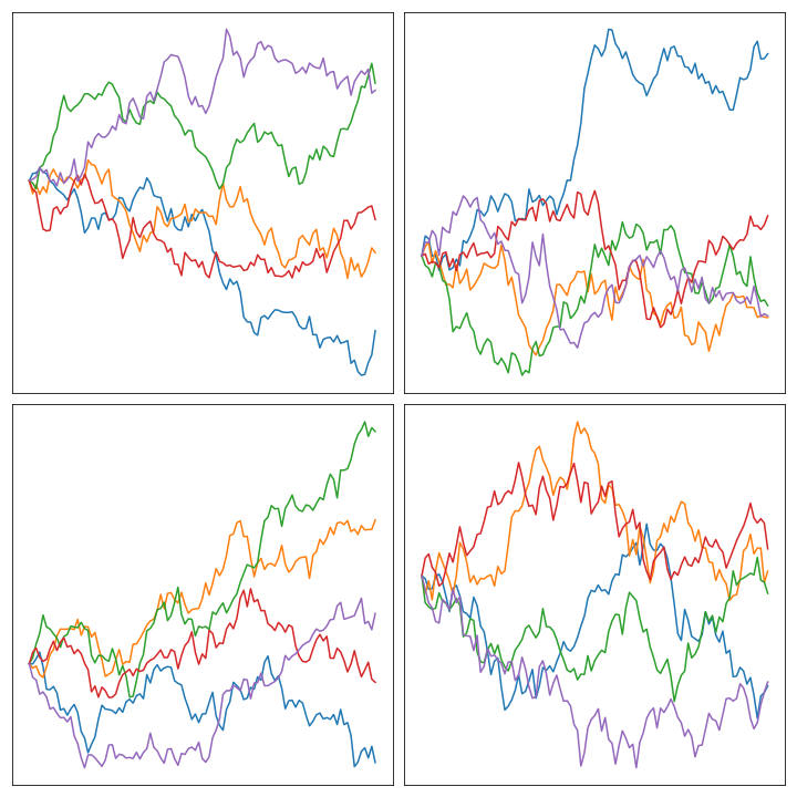
Here’s an image of the result of sampling some of them and plotting them in the unit interval:

Priors with bounded curvature #

A very similar procedure could be applied to the condition of bounded curvature. What we mean in this case is that the second derivative would be bounded by a given constant, say, again, \(\gamma\) . The condition of bounded second derivative can be written after discretization as \[ \left|\frac{X_{j-1} - 2X_{j} + X_{j+1}}{h^2}\right| < \gamma \] which, after solving for \(X_j\) , gives rise to the following system of equations:

\(n^2\begin{bmatrix}-2&1&& \\\phantom{-}1&-2&1& \\&\ddots&\ddots& \\&&1&-2 \\\end{bmatrix}\) \(\begin{bmatrix}X_1\\\vdots\\X_{n-1}\\\end{bmatrix} =\) \(\begin{bmatrix}\gamma W_1 - X_0\\\vdots\\\gamma W_{n-1} - X_n\\\end{bmatrix}\) .

An easy modification of create_L1 and bounded_slope can be used here in order to create L2 (assuming that the boundary points are 0) and to solve the system using this new matrix:

def create_L2(n):
    # Creating the diagonals
    diagonals = [
        [1]*n,
        [-2]*n,
        [1]*n
    ]

    # Specifying the offsets
    offsets = [-1, 0, 1]

    # Creating the matrix
    L2 = n ** 2 * sparse.diags(diagonals, offsets=offsets, shape=(n, n))
    return L2

def bounded_curvature(n, gamma):
    L2 = create_L2(n)

    # Sampling
    W = gamma * np.random.normal(size=(n, 1))
    
    # Solving the system
    X_interior = spsolve(L2, W)

    # Putting boundary conditions
    X = np.array([0, *X_interior, 0])
    return X

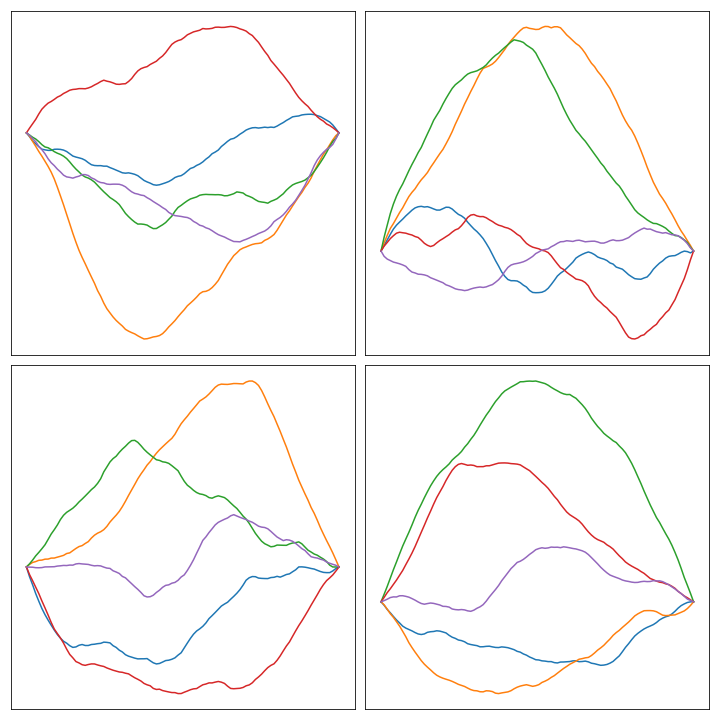
Notice that we’re refreshing the notation and using \(n\) instead of \(n-1\) . Here are some plots of the result of solving the linear system with \(L_2\) with some random draws:

Higher dimensions #

We can extend this line of reasoning to higher dimensions: instead of making assumptions about the first and second order derivatives of \(X:[0,1]\to\mathbb{R}\) , consider making assumptions about the Laplacian \(\Delta = \partial_{x_1}^2X + \partial_{x_2}^2X\) for \(X:[0,1]^2\to\mathbb{R}\) . In order to do so, we will need to construct a finite-difference approximation of the Laplacian, call it \(L_3\) . After that, it is as easy as considering the solutions of \(L_3X = W\) for \(X\) and \(W\) stacked vectors of size \(n^2\) .

Our life is made easier by the fact that discrete Laplacians can be constructed from the matrices we have already built above, as it turns out that discrete Laplacians are just Kronecker sums of the finite-difference operators for the second derivative in one dimension, that is, \(L_3 = I \otimes L_2 + L_2 \otimes I\) . We can compute these Kronecker products using sparse.kron:

def create_L3(n):
    # Getting L2
    L2 = create_L2(n)

    # Computing the Kronecker products
    D1 = sparse.kron(sparse.eye(n-1), L1)
    D2 = sparse.kron(L1, sparse.eye(n-1))
    
    # L3 as the sum of the products
    L3 = D1 + D2
    return L3

We can easily solve the system and un-stack the vector to get a matrix by reshaping:

def bounded_Laplacian(n, gamma):
    L3 = create_L3(n)

    # Sampling
    W = gamma * np.random.normal(size=(n ** 2, 1))

    X = spsolve(L3, W)

    # Ignoring boundary conditions
    return X.reshape((n, n))

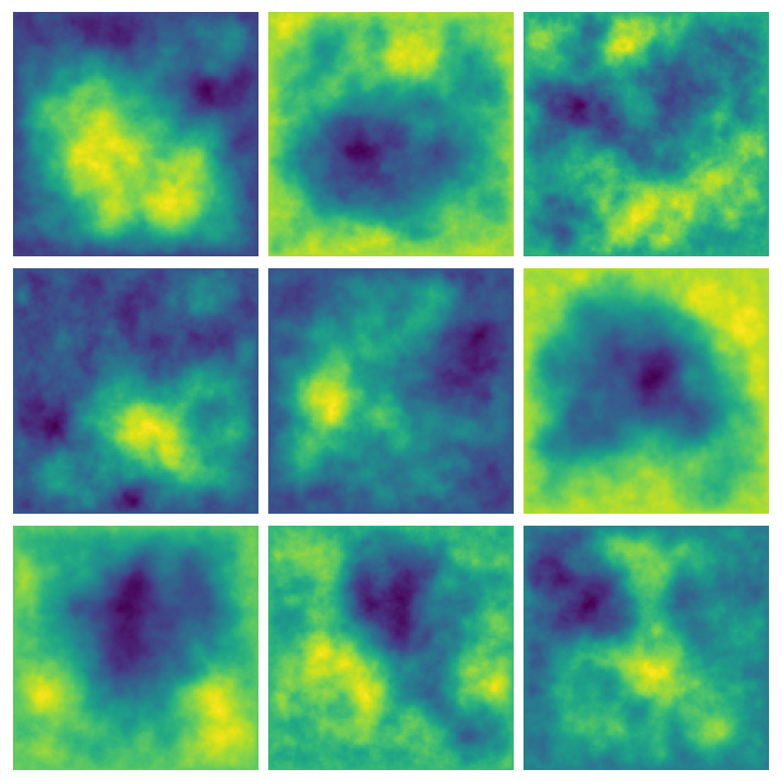
Here are some examples of multiple results of querying this function:

Whittle-Matérn priors #

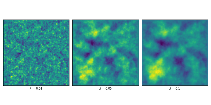
In order to introduce a measure of correlation, we can consider the finite-differences approximation of a different operator, given by the first derivate (or respectively the second) plus \(\lambda^{-2}\) times the identity. The priors that result from solving this finite-difference approximation are called Whittle-Matérn priors, and \(\lambda\) is called the correlation length.

In our code, it is as simple as constructing a new matrix \(L = L_i + \lambda^{-2}I\) for each \(i\) in \(\{1, 2, 3\}\) , depending on what we’re trying to build. In order to illustrate, I show a couple of results of sampling the solution to the problem using the 2D example (i.e. \(L = L_3 + \lambda^{-2}I\) ) and different lambdas.

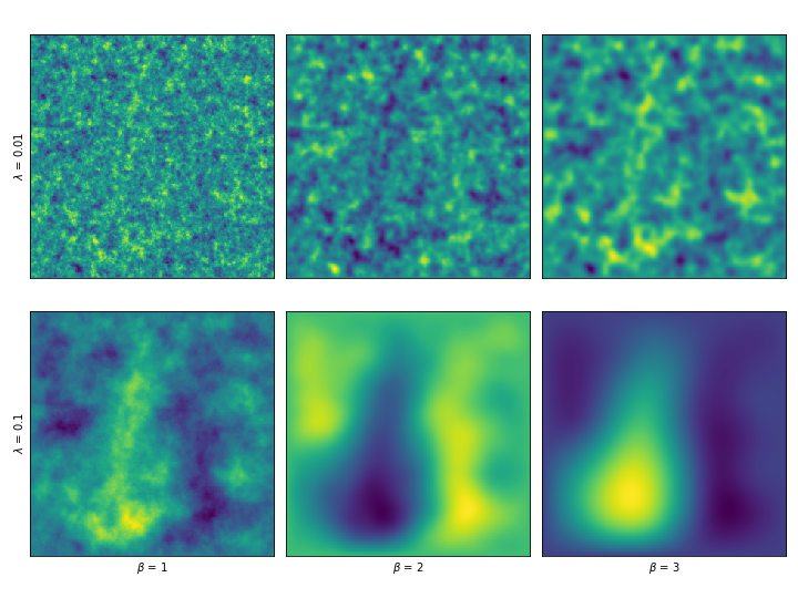
We can even introduce a smoothness order \(\beta\) by solving the system \(L^\beta X = \gamma W\) . By applying the operator more than once, we would be making assumptions about higher order derivatives. These are a couple examples, varying \(\beta\) and \(\lambda\) .

Conclusion and future directions #

This post discusses how to create priors for Bayesian processes. The method consists on assuming conditions on the function itself and approximate it in a grid. We discussed two examples in 1D: bounded first and second derivative. These assumptions and this approximation give rise to a system of linear equations of the form \(L_iX = \gamma W\) , where \(\gamma\) encodes the bound, \(L_i\) is the finite-difference approximation of the differential operator and \(W\) is sampled from a normal distribution with mean 0 and variance 1. We also discussed how this idea can be expanded to two dimensions by bounding the Laplacian of a function \(X:[0,1]^2\to\mathbb{R}\) .

We can expand the amount of free parameters we can tweak by considering Whittle-Matérn priors, in which a correlation length parameter \(\lambda\) is introduced and the system of equations changes to \((L_i + \lambda^{-2}I)X = \gamma W\) . Another parameter is introduced by considering the system \((L_i + \lambda^{-2}I)^\beta X = \gamma W\) , that is, by considering higher order derivatives.

Besides the use in scientific computing, I think these priors could be used as a source of noise for Procedural Content Generation, just like Perlin Noise is used to create artificial landscapes. I plan to explore this direction in future posts.

(All the code of this post, including image generation, can be found in this gist)